Blog

Learn R – Part 4

1. Basic Statistical Functions

R provides built-in functions for statistical analysis:

summary(): Summary statistics (min, max, quartiles, mean).

sum(): Total of values.

range(): Minimum and maximum.

var(): Variance.

sd(): Standard deviation.

Demo Data

# Basic dataset  
data_basic <- c(2, 4, 6, 8, 10)  
# Advanced dataset (mtcars)  
data(mtcars)  

mpg <- mtcars$mpg  

Practice

# BASIC TASKS  
# HW1: Calculate the sum of data_basic  
# HW2: Find the range (min and max) of data_basic  
# HW3: Compute the variance of data_basic  

# ADVANCED TASKS  
# HW4: Calculate the standard deviation of mtcars$mpg  

# HW5: Generate a summary of mtcars$hp (horsepower)  

Solution

# BASIC SOLUTIONS  
sum_basic <- sum(data_basic)  
range_basic <- range(data_basic)  
var_basic <- var(data_basic)  

# ADVANCED SOLUTIONS  
sd_mpg <- sd(mpg)  
summary_hp <- summary(mtcars$hp)  

2. Mean, Median, Mode

Mean : Average (mean()).

Median : Middle value (median()).

Mode : Most frequent value (no built-in function—custom code required).

Demo Data

# Basic dataset  
data_numbers <- c(1, 2, 2, 3, 4, 5, 5, 5)  
# Advanced dataset (iris)  
data(iris)  
sepal_length <- iris$Sepal.Length 

Practice

# BASIC TASKS  
# HW1: Calculate the mean of data_numbers  
# HW2: Find the median of data_numbers  
# HW3: Write a function to compute the mode  

# ADVANCED TASKS  
# HW4: Compute the mean of iris$Sepal.Length  

# HW5: Find the median of iris$Petal.Length grouped by Species  

Solution

# BASIC SOLUTIONS  
mean_val <- mean(data_numbers)  
median_val <- median(data_numbers)  
mode_func <- function(x) {  
  ux <- unique(x)  
  ux[which.max(tabulate(match(x, ux)))]  
}  
mode_val <- mode_func(data_numbers)  

# ADVANCED SOLUTIONS  
mean_sepal <- mean(sepal_length)  
median_petal <- aggregate(Petal.Length ~ Species, iris, median)  

3. Max, Min, and Percentiles

max()/min(): Extreme values.

quantile(): Percentiles (e.g., 25th, 50th).

IQR(): Interquartile range.

Demo Data

# Basic dataset  
data_scores <- c(45, 67, 89, 34, 56, 78, 90, 23)  
# Advanced dataset (airquality)  
data(airquality)  

temp <- airquality$Temp  

Practice

# BASIC TASKS  
# HW1: Find the max and min of data_scores  
# HW2: Calculate the 75th percentile of data_scores  
# HW3: Compute the IQR of data_scores  

# ADVANCED TASKS  
# HW4: Find the 90th percentile of airquality$Temp  

# HW5: Identify outliers in airquality$Ozone using IQR  

Solution

# BASIC SOLUTIONS  
max_score <- max(data_scores)  
min_score <- min(data_scores)  
percentile_75 <- quantile(data_scores, 0.75)  
iqr_score <- IQR(data_scores)  

# ADVANCED SOLUTIONS  
percentile_90 <- quantile(temp, 0.90)  
# Outlier detection (IQR method)  
q1 <- quantile(airquality$Ozone, 0.25)  
q3 <- quantile(airquality$Ozone, 0.75)  
iqr <- IQR(airquality$Ozone)  
outliers <- airquality$Ozone[airquality$Ozone < (q1 - 1.5*iqr) | airquality$Ozone > (q3 + 1.5*iqr)]  

4. Hypothesis Testing (T-Test/ANOVA)

Perform t-tests (t.test()), ANOVA (aov()), and chi-square tests (chisq.test()) to compare groups.

Demo Data

# Create sample data  
group_a <- c(20, 22, 19, 18, 24)  

group_b <- c(25, 24, 22, 23, 20)  

Practice

# HW1: Perform an independent t-test between group_a and group_b  

# HW2: Run a one-way ANOVA on `mtcars` to compare `mpg` across cylinder groups  

Solution

# HW1  
t.test(group_a, group_b)  
# HW2  
cyl_groups <- split(mtcars$mpg, mtcars$cyl)  
anova_result <- aov(mpg ~ factor(cyl), data=mtcars)  
summary(anova_result)  

5. Regression Analysis (Linear Regression)

Fit linear (lm()) and logistic regression models. Use summary() to interpret coefficients and p-values.

Demo Data

# Use `mtcars` for linear regression  

Practice

# HW1: Fit a linear model predicting `mpg` from `wt` and `hp`  

# HW2: Check the R-squared value of the model  

Solution

# HW1  
model <- lm(mpg ~ wt + hp, data=mtcars)  
# HW2  
summary(model)$r.squared  

6. Data Transformation

Recode variables with dplyr::mutate() and case_when(). Create new variables using arithmetic/logical operations.

Demo Data

# Create sample data  
df <- data.frame(  
  age = c(18, 25, 30, 35, 40),  
  income = c(50000, 60000, 75000, 90000, 120000) 
 
)  

Practice

# HW1: Recode `age` into categories: "<25", "25-35", ">35"  

# HW2: Create a new variable `income_group` (Low: <70k, High: >=70k)  

Solution

# HW1  
library(dplyr)  
df <- df %>%  
  mutate(age_group = case_when(  
    age < 25 ~ "<25",  
    age >= 25 & age <= 35 ~ "25-35",  
    age > 35 ~ ">35"  
  ))  
# HW2  
df <- df %>%  
  mutate(income_group = ifelse(income >= 70000, "High", "Low"))  

7. Exporting Results

Export tables and plots using write.csv(), stargazer, or flextable.

Practice

# HW1: Save `mtcars` summary to a CSV  

# HW2: Export a ggplot to PNG  

Solution

# HW1  
write.csv(summary(mtcars), "mtcars_summary.csv")  
# HW2  
ggsave("plot.png", plot=last_plot())  

8. Additional Statistical Concepts

Skewness : Measure of asymmetry (moments package).

Kurtosis : Tailedness of the distribution (moments package).

Covariance : cov().

Correlation : cor().

Demo Data

# Advanced dataset (cars)  
data(cars)  
speed <- cars$speed  

dist <- cars$dist  

Practice

# HW1: Calculate covariance between speed and distance  
# HW2: Compute correlation between speed and distance  

# HW3: Install the `moments` package and calculate skewness of speed  

Solution

# HW1  
covariance <- cov(speed, dist)  
# HW2  
correlation <- cor(speed, dist)  
# HW3  
library(moments)  
skewness_speed <- skewness(speed)  

9. Handling Missing Values

Use na.rm = TRUE to ignore NA values in calculations.

Demo Data

data_missing <- c(1, 2, NA, 4, 5)  

Practice

# HW1: Calculate the mean of data_missing (ignore NA)  

# HW2: Check if data_missing contains any NA values  

Solution

mean_missing <- mean(data_missing, na.rm = TRUE)  
has_na <- anyNA(data_missing)  

Learn R – Part 3

1. Plot (Data Visualization)

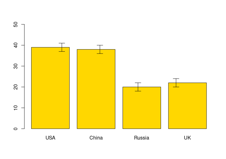
Plots visualize trends and relationships. Use plot() for basic graphs, lines()/points() for overlays, and par() for layouts. Customize with main, xlab, ylab, col, lwd, pch, and bg.

Demo Data (Basic)

# Simple dataset for beginners  
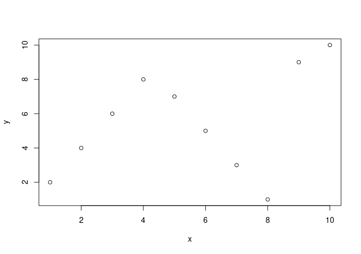
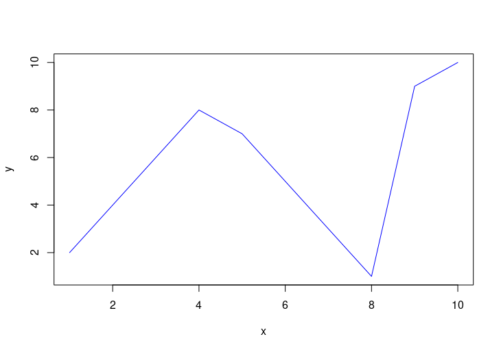
x <- 1:10  

y <- c(2, 4, 6, 8, 7, 5, 3, 1, 9, 10)  

Demo Data (Advanced)

# Complex dataset: mtcars (built-in)  
data(mtcars)  
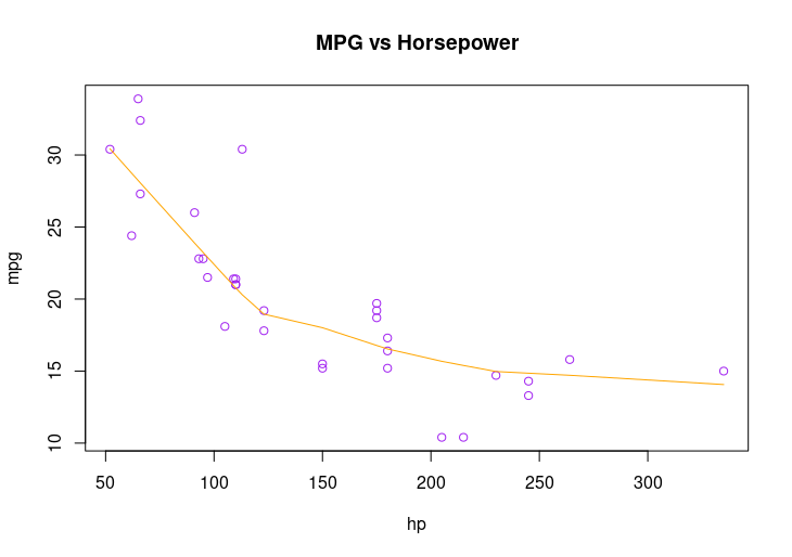
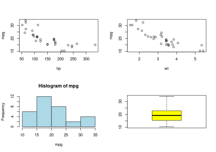
mpg <- mtcars$mpg  # Miles per gallon  
hp <- mtcars$hp    # Horsepower  

wt <- mtcars$wt    # Weight  

Practice

# BASIC TASKS  
# HW1: Plot x vs. y as points  
# HW2: Add a blue line to the plot  
# HW3: Create a plot with red triangles (pch=17)  

# ADVANCED TASKS  
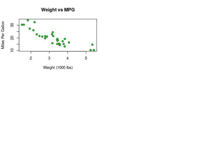
# HW4: Plot mpg vs. hp from mtcars, add a smooth line  
# HW5: Create a multi-plot layout (2x2 grid) 

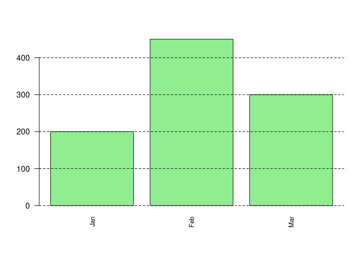
# HW6: Customize mpg vs. wt plot: title, axis labels, green points, gray background  

Solution

# BASIC SOLUTIONS  
plot(x, y)  
plot(x, y, type="l", col="blue")  
plot(x, y, pch=17, col="red")  

# ADVANCED SOLUTIONS  
plot(mpg ~ hp, data=mtcars, main="MPG vs Horsepower", col="purple")  
lines(lowess(hp, mpg), col="orange")  

par(mfrow=c(2,2))  
plot(mpg ~ hp, data=mtcars)  
plot(mpg ~ wt, data=mtcars)  
hist(mpg, col="lightblue")  
boxplot(mpg, col="yellow")  

plot(mpg ~ wt, data=mtcars,  
     main="Weight vs MPG",  
     xlab="Weight (1000 lbs)",  
     ylab="Miles Per Gallon",  
     pch=21, bg="green",  
     panel.first=grid())  

2. Pie Chart

Pie charts show proportions. Use pie(), legend(), and ifelse() for conditional formatting.

Demo Data (Basic)

# Simple sales data  
sales <- c(25, 35, 40)  

labels <- c("Apparel", "Electronics", "Groceries")  

Demo Data (Advanced)

# Complex dataset: Titanic survival rates  
survivors <- c(203, 118, 178, 528)  

groups <- c("1st Class", "2nd Class", "3rd Class", "Crew")  

Practice

# BASIC TASKS  
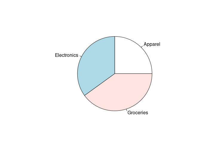
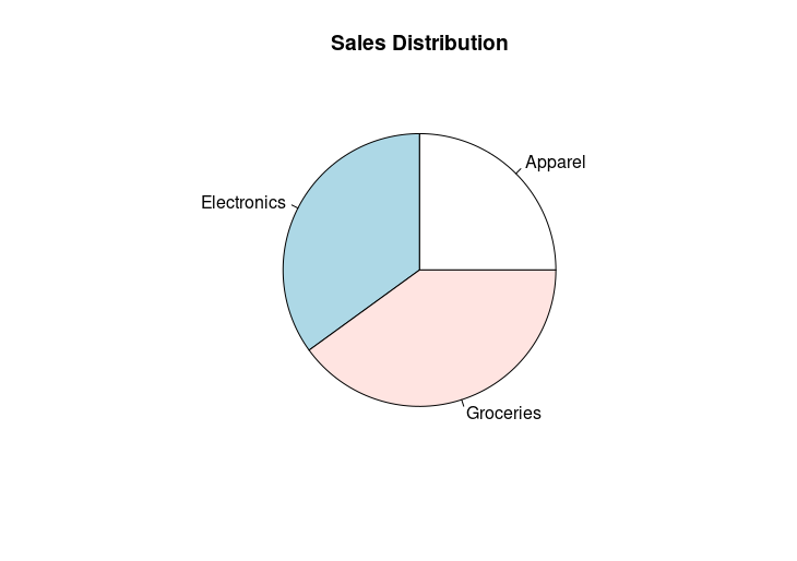
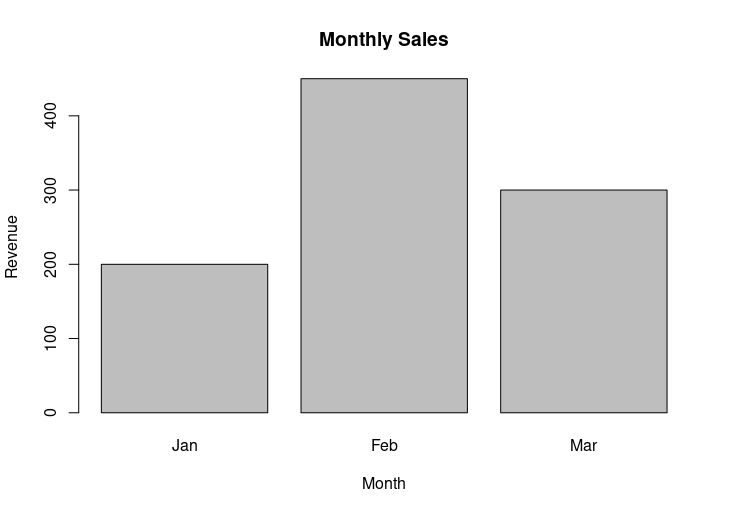
# HW1: Create a pie chart for sales data  
# HW2: Add a title and explode the "Groceries" slice  

# ADVANCED TASKS  
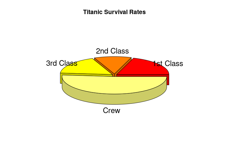
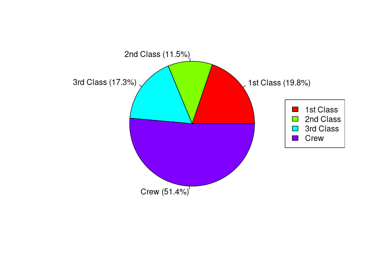
# HW3: Plot Titanic survival rates with gradient colors  
# HW4: Add a legend and percentage labels  

# HW5: Create a 3D pie chart (use plotrix package)  

Solution

# BASIC SOLUTIONS  
pie(sales, labels=labels)  
pie(sales, labels=labels, main="Sales Distribution", explode=0.1)  

# ADVANCED SOLUTIONS  
# Install the plotrix package (only needed once)
install.packages("plotrix")

# Load the package
library(plotrix)

library(plotrix)  
pie3D(survivors, labels=groups, main="Titanic Survival Rates",  
      col=heat.colors(4), explode=0.05)  

pie(survivors, labels=paste(groups, " (", round(survivors/sum(survivors)*100, 1), "%)", sep=""),  
    col=rainbow(4))  
legend("right", groups, fill=rainbow(4))  

3. Bar Chart

Bar charts compare categories. Use barplot(), beside=TRUE for grouped bars, and col for gradients.

Demo Data (Basic)

# Monthly sales  
months <- c("Jan", "Feb", "Mar")  

sales <- c(200, 450, 300)  

Demo Data (Advanced)

# Complex dataset: Olympic medal counts  
countries <- c("USA", "China", "Russia", "UK")  
gold <- c(39, 38, 20, 22)  
silver <- c(41, 32, 28, 21)  

bronze <- c(33, 18, 23, 22)  

Practice

# BASIC TASKS  
# HW1: Create a vertical bar chart for monthly sales  
# HW2: Add grid lines and rotate labels  

# ADVANCED TASKS  
# HW3: Create stacked bars for Olympic medals  
# HW4: Create grouped bars with legends  

# HW5: Add error bars using arrows()  

Solution

# BASIC SOLUTIONS  
barplot(sales, names.arg=months, main="Monthly Sales", xlab="Month", ylab="Revenue")  
barplot(sales, names.arg=months, las=2, cex.names=0.8, col="lightgreen")  
abline(h=seq(0, 500, by=100), lty=2)  

# ADVANCED SOLUTIONS  
medals <- rbind(gold, silver, bronze)  
barplot(medals, names.arg=countries, col=c("gold", "silver", "darkorange"),  
        legend=rownames(medals), main="Olympic Medals", beside=TRUE)  

# Error bars  
barplot(gold, names.arg=countries, ylim=c(0, 50), col="gold")  
arrows(x0=1:4, y0=gold-2, y1=gold+2, code=3, angle=90, length=0.1)  

Learn R – Part 2

1. Vectors

Vectors are 1D data structures holding elements of the same type .

Sort : sort() (ascending) or rev(sort()) (descending).

Create : Use c(), seq(from, to, by), or rep(value, times).

Access : Use [index] (positive/negative), logical vectors, or names.

Length : length(vector).

# HW1: Create a vector of even numbers 2, 4, 6 using `seq()`  
# HW2: Access the 3rd element of `c(10, 20, 30, 40)`  
# HW3: Sort `c(5, 1, 3)` in descending order  
# HW4: Check the length of `c("a", "b", "c")`  

# HW5: Create a vector with 3 copies of "R" using `rep()`  

# HW1  
vec_seq <- seq(2, 6, by=2)  # Output: 2, 4, 6  
# HW2  
print(c(10, 20, 30, 40)[3])  # Output: 30  
# HW3  
sorted <- rev(sort(c(5, 1, 3)))  # Output: 5, 3, 1  
# HW4  
print(length(c("a", "b", "c")))  # Output: 3  
# HW5  
vec_rep <- rep("R", 3)  # Output: "R", "R", "R"  

2. Lists

Lists store mixed or nested data .

Add/Remove : list[[new_index]] <- value or list[index] <- NULL.

Create : list().

Access : [index] (returns sublist), [[index]] (returns element), or $name.

Modify : Assign new values via [[ ]] or append().

# HW1: Create a list with "apple", 25, and a sub-list `c(1, 2)`  
# HW2: Access the sub-list `c(1, 2)` from HW1  
# HW3: Change "apple" to "banana" in the list  
# HW4: Add `TRUE` to the end of the list  

# HW5: Remove the 2nd element (25)  

# HW1  
my_list <- list("apple", 25, list(1, 2))  
# HW2  
print(my_list[[3]])  # Output: 1, 2  
# HW3  
my_list[[1]] <- "banana"  
# HW4  
my_list <- append(my_list, TRUE)  
# HW5  
my_list[2] <- NULL  

3. Matrices

Matrices are 2D, same-type data structures.

Generate Values : seq(), rep().

Create : matrix(data, nrow, ncol).

Access : [row, col], [,] for entire rows/columns.

Add Rows/Columns : rbind(), cbind().

# HW1: Create a 3x2 matrix with 1-6 using `matrix()`  
# HW2: Extract the 2nd row  
# HW3: Extract the 1st column  
# HW4: Add a row `7, 8` to the matrix  

# HW5: Create a matrix with 1, 2 repeated 3 times using `rep()`  

# HW1  
mat <- matrix(1:6, nrow=3)  
# HW2  
print(mat[2, ])  # Output: 2, 5  
# HW3  
print(mat[, 1])  # Output: 1, 2, 3  
# HW4  
mat <- rbind(mat, c(7, 8))  
# HW5  
mat_rep <- matrix(rep(1:2, 3), nrow=3)  

4. Arrays

Arrays extend matrices to multi-dimensional data .

Dimensions : dim() to check or set dimensions.

Create : array(data, dim=c(rows, cols, ...)).

Access : [i, j, k] for specific elements.

# HW1: Create a 2x2x2 array with values 1-8  
# HW2: Access the 3rd element of the 1st layer  
# HW3: Extract the 2nd layer (all rows/columns)  
# HW4: Check the total length of the array  

# HW5: Convert a vector `1:12` into a 3x4 array  

# HW1  
arr <- array(1:8, dim=c(2, 2, 2))  
# HW2  
print(arr[3])  # Output: 3  
# HW3  
print(arr[, , 2])  
# HW4  
print(length(arr))  # Output: 8  
# HW5  
arr_3d <- array(1:12, dim=c(3, 4))  

5. Data Frames

Data frames store tabular data (mixed types allowed).

Modify : Add/remove columns via $ or [ ].

Create : data.frame().

Access : $column, [, "column"], or subset().

# HW1: Create a data frame with Name (Alice, Bob), Age (25, 30)  
# HW2: Access the "Name" column using `$`  
# HW3: Add a column "Salary" with 5000, 6000  
# HW4: Remove the "Age" column  

# HW5: Check the number of rows  

# HW1  
df <- data.frame(Name=c("Alice", "Bob"), Age=c(25, 30))  
# HW2  
print(df$Name)  # Output: Alice, Bob  
# HW3  
df$Salary <- c(5000, 6000)  
# HW4  
df$Age <- NULL  
# HW5  
print(nrow(df))  # Output: 2  

6. Factors

Factors store categorical data with predefined levels.

Ordered Factors : ordered=TRUE for ranking.

Create : factor().

Modify Levels : levels(), factor(..., levels=).

# HW1: Create a factor with "Low", "Medium", "High"  
# HW2: Check the levels of the factor  
# HW3: Add "Very High" as a new level  
# HW4: Remove "Medium" from the factor  

# HW5: Convert the factor to an ordered factor  

# HW1  
f <- factor(c("Low", "Medium", "High"))  
# HW2  
print(levels(f))  # Output: "High", "Low", "Medium"  
# HW3  
f <- factor(f, levels=c("Low", "Medium", "High", "Very High"))  
# HW4  
f <- f[f != "Medium"]  
# HW5  
f_ordered <- factor(f, ordered=TRUE)  

Learn R – Part 1

1. How to Write an R Code (Syntax and Print)

R uses simple syntax to execute commands. Code is written line-by-line, and print() or cat() displays output. Try, if you can solve the below problem.

# HW 1: Print "Hello, R!"  

# HW 2: Calculate 5 + 3 and print the result  

print("Hello, R!")  
cat("Result:", 5 + 3)  

2. To See a Data Type

Use class() / typeof() to check the data type of a variable (e.g., numeric, character).

# HW 1: Check the type of "apple"  

# HW 2: Check the type of 25.6  

class("apple")  # Output: "character"  
typeof(25.6)     # Output: "double"  

3. To Set a Data Type

Use as. function to set forcefully a data type like as.numeric() or as.character().

# HW 1: Convert "100" to numeric  

# HW 2: Convert 50 to character  

as.numeric("100")  # Output: 100  
as.character(50)   # Output: "50"  

4. To Handle Multiple values at once

Use vectors (created with c()) to store multiple values of the same type.

# HW 1: Create a vector of numbers 1, 2, 3  

# HW 2: Create a vector of colors: "red", "blue"  

nums <- c(1, 2, 3)  
colors <- c("red", "blue")  

5. To Define a Value

Assign values to variables using <- or =. Example: x <- 10.

# HW 1: Assign 3.14 to "pi"  

# HW 2: Assign "Rocks" to "language"  

pi <- 3.14  
language <- "Rocks"  

6. How to make a Comment

Use # to add comments (notes) to your code. R ignores these lines.

# HW 1: Write a comment explaining the next line  

  print("Learning R!")  

# This line prints a motivational message  
print("Learning R!")  

7. Variables and Their Types

Variables in R store data, and their type is automatically inferred from the assigned value. Use <- or = to assign values. Example: x <- 10 (numeric), y <- "Hello" (character).

# HW1: Assign 3.14 to a variable  
# HW2: Assign "R Programming" to a variable  

# HW3: Assign TRUE to a variable  

pi_value <- 3.14  
language <- "R Programming"  
is_fun <- TRUE  

8. Different Data Types in R

R supports numeric (e.g., 10.5), integer (e.g., 55L), complex (e.g., 9+3i), character (e.g., "R is exciting"), and logical (e.g., TRUE). Use class() to check the type.

# HW1: Create a numeric variable with 787  
# HW2: Create an integer with 100L  
# HW3: Create a complex number 9+3i  
# HW4: Create a character "FALSE"  

# HW5: Create a logical FALSE  

num <- 787  
integer_val <- 100L  
complex_num <- 9 + 3i  
char <- "FALSE"  
logical_val <- FALSE  

9. Simple Math Functions

R has built-in functions for math operations:

min(): Finds the smallest value.

floor(): Rounds down to the nearest integer.

max(): Finds the largest value.

sqrt(): Calculates the square root.

abs(): Returns absolute value.

ceiling(): Rounds up to the nearest integer.

# HW1: Find the minimum of 10, 20, 5  
# HW2: Calculate the square root of 16  
# HW3: Round 3.2 up and 4.9 down  

# HW4: Get the absolute value of -7.5  

min_val <- min(10, 20, 5)  # Output: 5  
sqrt_val <- sqrt(16)       # Output: 4  
ceil_val <- ceiling(3.2)   # Output: 4  
floor_val <- floor(4.9)    # Output: 4  
abs_val <- abs(-7.5)       # Output: 7.5  

10. Boolean’s (Logical Values)

Booleans are TRUE or FALSE. Use logical operators like & (AND), | (OR), and ! (NOT) to combine conditions.

# HW1: Check if 5 > 3 AND 2 < 4 
# HW2: Check if 10 == 10 OR 7 != 7  

# HW3: Reverse the value of TRUE  

bool1 <- (5 > 3) & (2 < 4)
bool1   # Output: TRUE  
bool2 <- (10 == 10) | (7 != 7)
bool2   # Output: TRUE  
bool3 <- !TRUE  
bool3   # Output: FALSE  

11. Arithmetic Operators

Used for basic math operations: + (add), - (subtract), * (multiply), / (divide), ^ (exponent), %% (modulus).

# HW1: Calculate 10 + 5  
# HW2: Calculate 10 - 5  
# HW3: Calculate 4 * 6  
# HW4: Calculate 20 / 4  
# HW5: Calculate 3^2 (3 squared)  

# HW6: Find the remainder of 10 %% 3  

add <- 10 + 5   # 15  
sub <- 10 - 5   # 5  
mul <- 4 * 6    # 24  
div <- 20 / 4   # 5  
exp <- 3^2      # 9  
mod <- 10 %% 3  # 1  

12. Assignment Operators

Assign values to variables: <-, =, or -> (rarely used). Example: x <- 5 or 5 -> x.

# HW1: Assign 10 to `a` using `<-`  
# HW2: Assign 20 to `b` using `=`  

# HW3: Assign 30 to `c` using `->`  

a <- 10  
b = 20  
30 -> c  

Compare values: == (equal), != (not equal), >, <, >=, <=. Returns TRUE or FALSE.

# HW1: Check if 5 == 5  
# HW2: Check if 10 != 5  
# HW3: Check if 8 > 3  

# HW4: Check if 4 <= 4  

5 == 5    # TRUE  
10 != 5  # TRUE  
8 > 3     # TRUE  
4 <= 4   # TRUE  

14. Logical Operators

Combine conditions: & (AND), | (OR), ! (NOT).

# HW1: Check if (5 > 3) & (2 < 4)  
# HW2: Check if (10 == 5) | (3 != 3)  

# HW3: Reverse the result of TRUE using `!`  

(5 > 3) & (2 < 4)  # TRUE  
(10 == 5) | (3 != 3)  # FALSE  
not_op <- !TRUE  
not_op    # FALSE  

15. If-Else Statements

Use if to execute code if a condition is TRUE, and else for when it’s FALSE.

# HW1: Check if 10 is greater than 5, print "Yes"  
# HW2: Check if 7 is even; if not, print "Odd"  

# HW3: Assign "Pass" if score >= 50, else "Fail"  

# HW1  
if (10 > 5) {  
  print("Yes")  
}  

# HW2  
if (7 %% 2 == 0) {  
  print("Even")  
} else {  
  print("Odd")  
}  

# HW3  
score <- 55  
result <- if (score >= 50) "Pass" else "Fail"  
print(result)  

16. While Loop

Repeats code while a condition is TRUE. Use break to exit early.

# HW1: Print numbers 1 to 5  

# HW2: Sum numbers from 1 to 3  

# HW1  
i <- 1  
while (i <= 5) {  
  print(i)  
  i <- i + 1  
}  

# HW2  
total <- 0  
j <- 1  
while (j <= 3) {  
  total <- total + j  
  j <- j + 1  
}  
print(total)  # Output: 6  

17. For Loop

Iterates over a sequence (like a vector). Use break/next to control flow.

# HW1: Print numbers 1 to 3 from c(1, 2, 3)  
# HW2: Calculate sum of 1, 2, 3 using a loop  

# HW3: Loop through a matrix (2x2) and print values  

# HW1  
for (num in c(1, 2, 3)) {  
  print(num)  
}  

# HW2  
sum <- 0  
for (i in 1:3) {  
  sum <- sum + i  
}  
print(sum)  # Output: 6  

# HW3  
mat <- matrix(1:4, nrow=2)  
for (row in 1:nrow(mat)) {  
  for (col in 1:ncol(mat)) {  
    print(mat[row, col])  
  }  
}  

18. Functions

Reusable code blocks. Use function() to define, and return() to output results.

# HW1: Create a function to square a number  

# HW2: Create a function that says "Hello, [name]!"  

# HW1  
square <- function(x) {  
  return(x^2)  
}  
print(square(4))  # Output: 16  

# HW2  
greet <- function(name) {  
  return(paste("Hello,", name, "!"))  
}  
print(greet("Alice"))  # Output: "Hello, Alice!"  

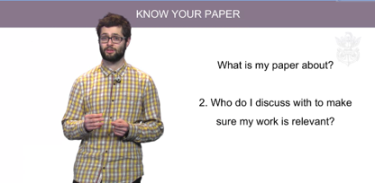
Course Review: How to Write and Publish a Scientific Paper

Recently, I completed the Coursera course “How to Write and Publish a Scientific Paper.” As someone new to research, I found this course incredibly valuable for building a strong foundation. It breaks down the research process step by step, from understanding the basics to confidently preparing your work for publication.

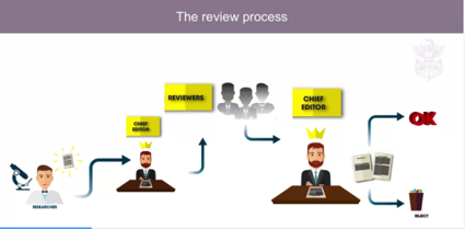
The course covers essential topics like structuring your paper, choosing the right journal, and navigating the peer-review process. What stood out most to me was how beginner-friendly yet comprehensive the lessons were—perfect for anyone starting their research journey.

If you’re looking to demystify academic writing and take your first step into the world of publishing, I highly recommend this course.

Link to the Course

Course Overview

This project-centered course is meticulously designed to lead students through the entire process of writing and publishing a scientific paper. It encompasses:

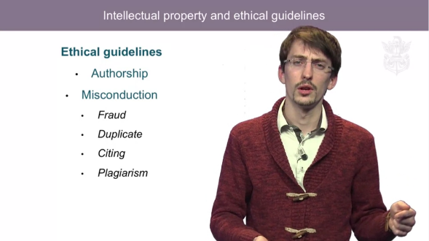
• Understanding Academia: Provides insights into the academic publishing landscape, including how scientific journals operate and the ethical considerations involved.
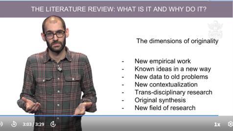
• Delimiting Your Scientific Paper: Guides on defining the scope and structure of your paper, ensuring clarity and focus.
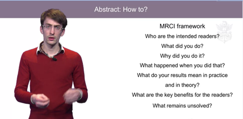
• Writing the Paper: Offers practical advice on crafting each section of the manuscript, from the introduction to the conclusion, and emphasizes the importance of proper citation practices.
• Post-Writing Checklist: Equips students with a comprehensive checklist to self-assess their work before submission, enhancing the likelihood of acceptance.

Personal Experience

As a novice in the research domain, I found this course to be exceptionally beneficial. The step-by-step approach demystified the complexities of scientific writing. The emphasis on ethical considerations and the peer-review process provided a holistic understanding of academic publishing. The practical assignments, particularly outlining a complete scientific paper and selecting an appropriate journal for submission, were instrumental in reinforcing the concepts learned.

Here are some interesting screenshots of the course that you might find interesting ;

Screenshot Credit: Coursera

For any kind of Query or problem feel free to contact me in my Email